BGL Technical Notes

Fault seal analysis: sensitivity to modelling methods and uncertainty therein.

Abstract
A significant proportion of the world’s conventional petroleum reservoirs occur in structural traps. Therefore, understanding the controls on structural geometry and fault seal are crucial steps in modelling/predicting hydrocarbon accumulation. One of the principal mechanisms by which faults are fluid-retaining is membrane seal; this is where smeared ‘clay minerals’ form impermeable barriers along structural planes. The following study shows that estimates of fault seal can be highly sensitive to the type of methods used to model the fault rock properties. Three methods were employed: B-Spline; SGS and a combined SGS+MPS method. The results suggest that, given the same structural model and well data, the pattern of fault seal integrity along the fault plane can vary considerably depending on the method used. Furthermore, stochastic methods (SGS and SGS+MPS) illustrate how uncertainty associated with the reservoir attributes (fault rock properties) propagate through to the final fault seal model. Therefore, uncertainties in fault seal estimates are fundamentally related to uncertainty in the faulted rock properties. The use of stochastic methods also helped illustrate the point that fault seal and reservoir properties are ‘coupled’ in an inverse sense so that fault seal will improve at the expense of reservoir quality.

Keywords: geostatistics, T7, fault seal, sensitivity, uncertainty

Click here to download PDF

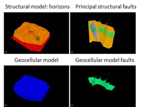	Figure 1. Principal components of the structural model and the derived geocellular model.
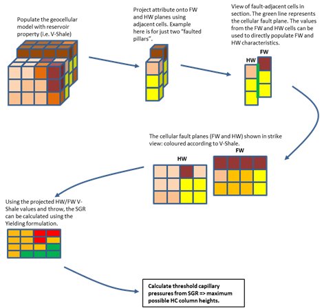	Figure 2. The generalised fault attribute modelling workflow. The entire workflow is automated, so once the model parameters are set the process.
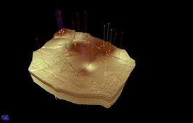	Figure 3. The B-Spline VShale reservoir property model. The wells have been included as a guide to their distribution and density. The same wells are used for all other methods.
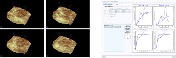	Figure 4. Four SGS realisations (from a possible 50) of modelled VShale. To the right, the experimental variograms and fitted models used for the SGS workflow. Note that the variography and SGS modelling was carried out in topological space to ensure depositional changes in V-Shale were preserved across faults.
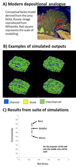	Figure 5. Summary of lithofacies modelling approach. A) The modern analogue used to inform the training image and conceptual model. B) Four MPS realisations (from a possible 50) lithofacies models. C) Connectivity vs Net:Gross plot for the 50 simulated models.
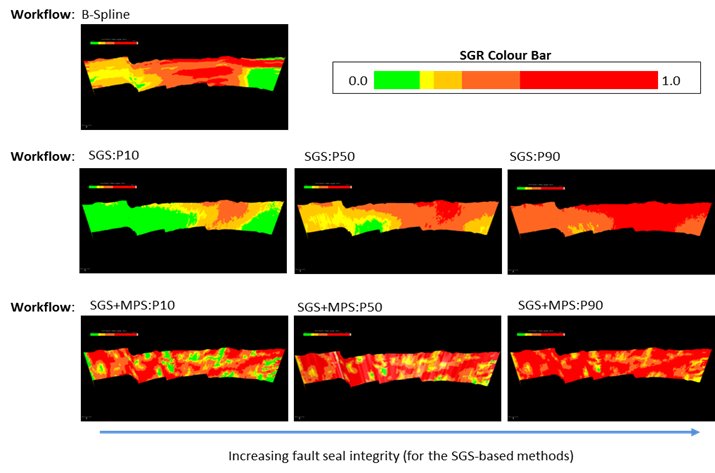	Figure 6. The SGR results for the main fault. Note the difference in SGR patterns between the three workflows. Most noteworthy, is the discrete lenticular nature of the SGS+MPS approach, highlighting the sensitivity of modelled SGR to reservoir architecture. The range of results for the stochastic methods (three cases are shown), also illustrates the need to appreciate the degree of uncertainty associated with reservoir VShale values and how these translate into fault attributes.
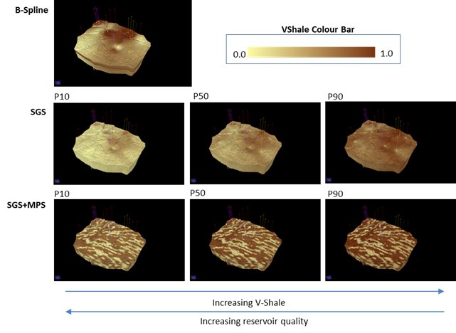	Figure 7. Summary diagram of the main findings of the VShale property modelling step. Three scenarios are selected from the SGS and SGS+MPS simulations. The choice of percentile cases (P10, P50 and P90) were chosen in order to capture both central tendency and end members implied from the range of uncertainty captured (per cell) by the suite of stochastic simulations.
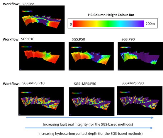	Figure 8. Overview of the hydrocarbon (HC) column heights computed via the SGR models, produced using the three different workflows, for all the cellular faults. Again one should note significant changes in the pattern of HC column height depending on the modelling method used and associated uncertainty as captured by the stochastic workflows. HC column heights are computed using the methods presented in Bretan et al. (2003).